By the Higher Math Guide editorial team. Last reviewed: 20 November 2026.
Calculator · Runs offline in your browser · Educational only · Updated 20 Nov 2026
Educational tool; results are estimates for learning, verify with your textbook or instructor.
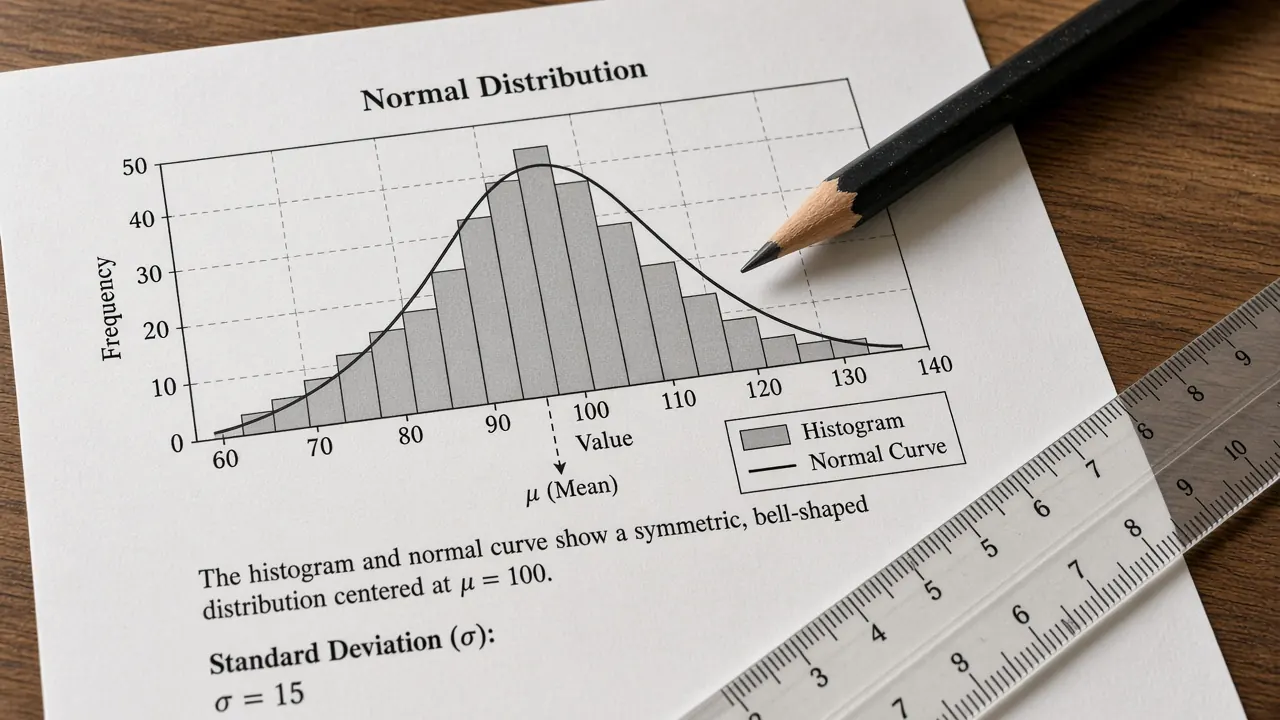
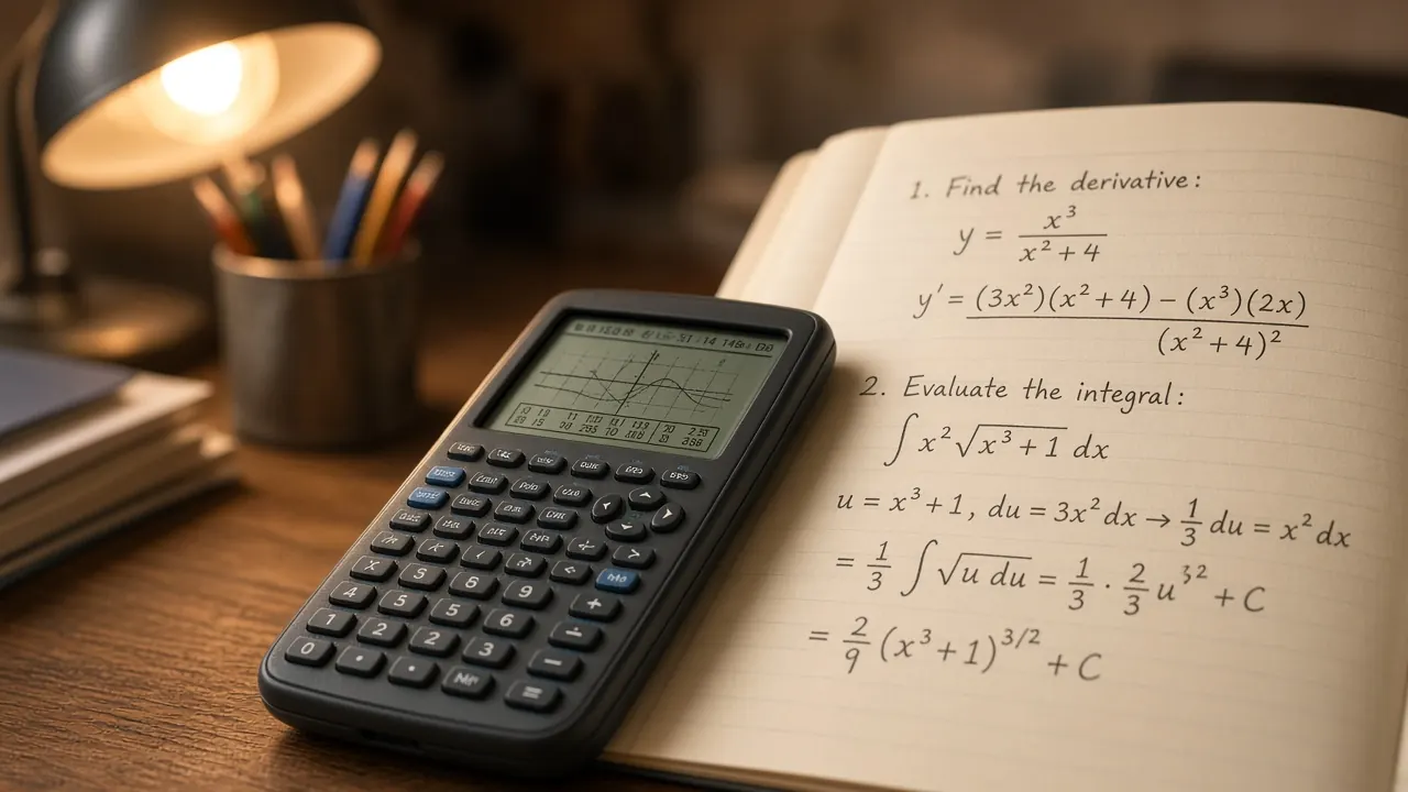
Counts, a curve, and a calculator, the setting for a Bayes update. Source
This tool computes a posterior for a yes or no hypothesis. You give a prior $P(H)$, a likelihood $P(E\mid H)$, and the chance of the same evidence when the hypothesis is false, $P(E\mid \text{not }H)$. It reports
and $P(\text{not }H)=1-P(H)$. The large number on the page is $P(H\mid E)$. The lines under it are the same formula with your inputs plugged in, including the two pieces that add up to $P(E)$.
The number is meaningful when $H$ and its opposite are the only two possibilities you are willing to consider, when the three inputs are probabilities in that same model, and when $E$ is the evidence you actually observed. A classroom test, a spam flag, or a card draw can fit once you name those events. A binomial count is a different job. That tool fixes a success probability and asks for the chance of exactly $k$ successes. Here those rates are inputs, and the output is an updated belief.
This is one update for one binary hypothesis. It does not estimate a prior from a data file, and it does not check that a later observation is independent of this one. Name the events in the Bayes theorem explainer before you trust a digit.
How to use the two input styles
Probability style is the formula as written. Enter $P(H)$, $P(E\mid H)$, and $P(E\mid \text{not }H)$, each in $[0,1]$, then press Compute. The defaults are a rare hypothesis: prior $0.01$, likelihood $0.99$, and a $0.05$ chance of the evidence when $H$ is false. That is the classroom test from the Bayes explainer, written as probabilities instead of a hall of people.
Natural frequency style replaces the prior with a head count. Enter a population size $N$, how many of those $N$ have $H$, and the same two likelihoods. The page sets $P(H)$ equal to the count divided by $N$, then runs the same formula. It also prints the expected true positive count and the expected false positive count, so you can see which group is supplying the evidence. The defaults are $N=10000$ and $100$ people with $H$, which is the same prior $0.01$. Those counts are expectations. If the rates do not land on whole people, the page still uses the exact ratio for the posterior.
Type probabilities as decimals. $0.99$ means 99 percent, and $99$ is rejected. Switching to counts rounds $P(H)\times N$ to a whole person. A repeating prior can move by about one person, so keep an exact decimal in probability style.
How to read the output
The large number is $P(H\mid E)$. When it is not a short decimal, it is rounded to 6 places and the word “about” appears with a percent. The lines underneath keep more digits. They are the same formula, not a second model.
$P(\text{not }H)$ is one minus the prior. The next two lines are the pieces before you divide: evidence from $H$, and evidence from the opposite. Their sum is $P(E)$. Dividing the piece from $H$ by that sum is the posterior. The other piece over the same sum is $P(\text{not }H\mid E)$. Those two posteriors add to $1$.
On the defaults, the piece from $H$ is $0.0099$ and the piece from the opposite is $0.0495$. So $P(E)=0.0594$ and
A bit under 17 percent, not $0.99$. Most of that evidence is false positives from the large group without $H$. Quoting the likelihood as if it were the posterior is base rate neglect. Count mode with $10000$ people prints $99$ expected true positives and $495$ expected false positives, and $99/(99+495)$ is the same $1/6$. If both likelihoods are positive and the prior sits strictly between $0$ and $1$, the page also prints the likelihood ratio and the prior and posterior odds. That is the same fraction in another form. If $P(E\mid H)$ is smaller than $P(E\mid \text{not }H)$, the posterior falls below the prior. That is a real update, not a broken input.
A second check you can do by hand
Two jars, from the probability and statistics topic. The prior on jar 1 is $1/2$. Jar 1 produces red with probability $3/4$, and jar 2 with probability $1/4$. Enter prior $0.5$, likelihood $0.75$, and $0.25$ for $P(E\mid \text{not }H)$. The posterior for jar 1 given red is $0.75$. The match with the likelihood is an accident of these counts. Change the prior to $0.1$ and leave the likelihoods alone. The posterior drops to $0.25$. If you still get $0.75$, you ignored the prior.
A third check in exact fractions
This one was added on 20 November 2026 and checked by hand, not by the screen. Take prior $P(H)=1/5$, likelihood $P(E\mid H)=1/2$, and $P(E\mid \text{not }H)=1/4$. Then $P(\text{not }H)=4/5$ and
The other posterior is $2/3$, and the two posteriors add to $1$. In odds, the prior odds are $(1/5)/(4/5)=1/4$, the likelihood ratio is $(1/2)/(1/4)=2$, and the posterior odds are $(1/4)\cdot 2=1/2$, which is the same statement as a posterior of $1/3$. Type prior $0.2$, likelihood $0.5$, and $0.25$ for the false positive rate. The large number should be $0.333333$, with the word about, because $1/3$ is not a short decimal. If the page prints $0.5$, it reported the likelihood and ignored the prior.
The short form of the update, next to conditional probability.
Sources checked 20 November 2026
OpenIntro Statistics, open textbook, conditional probability and Bayes. openintro.org/book/os (accessed 20 Nov 2026). The formula on this page is the standard update $P(H\mid E)=P(E\mid H)P(H)/P(E)$, with $P(E)$ expanded over $H$ and its opposite. The three numerical checks above are this site's arithmetic, not a copied textbook exercise.
The paired explainer, Bayes theorem without the fog, works the default inputs as counts in a hall of $10{,}000$ people. Rechecked against this calculator on 20 Nov 2026: prior $0.01$, likelihood $0.99$, and $P(E\mid \text{not }H)=0.05$ still give $0.0099/0.0594=1/6$.
Last reviewed: 20 November 2026.
Common pitfalls
$P(E\mid H)$ and $P(H\mid E)$ are different questions. Sensitivity is about the evidence given the hypothesis. The posterior is about the hypothesis given the evidence. The labels stay in one order. The button will not swap a story you told backwards.
A probability outside $[0,1]$ is rejected, and so is a head count larger than the population, a population below $1$, or a blank box. If $P(E)=0$, the posterior is undefined and the page stops instead of dividing by zero. A prior of $0$ stays $0$ when the evidence can still come from the opposite hypothesis. A prior of $1$ stays $1$ when the evidence can come from $H$. Population size stops at one billion.
The tool is binary: one hypothesis and its opposite. The three box card problem in the explainer has three priors, so do not fold those boxes into a single $H$ until you have decided which event $H$ is. A second observation needs its own likelihood. Feed the posterior back in as the next prior only when the new evidence is independent of the old evidence given $H$. The explainer shows a card draw where that independence fails.
A fixed number of independent trials with a constant success probability belongs on the binomial probability calculator. Counting selections, without a probability model, is the combinatorics calculator. A continuous tail is the normal CDF and z score calculator. None of those three updates a prior. This page does, and only for the binary hypothesis you type.
It returns $P(H\mid E)$, the posterior. You enter the prior $P(H)$, the likelihood $P(E\mid H)$, and $P(E\mid \text{not }H)$. The page also shows $P(E)$, the part of that evidence that comes from $H$, the part that comes from the opposite, and the posterior on not $H$.
Why can a sensitive test still leave a small posterior?
A headline accuracy is usually the likelihood, $P(E\mid H)$. If the hypothesis is rare, false positives from the large group without $H$ can outnumber the true positives. The defaults on this page do that. A prior of $0.01$ and a likelihood of $0.99$, with $P(E\mid \text{not }H)$ equal to $0.05$, produce a posterior of $1/6$, a bit under 17 percent.
Is P(E given H) the same as P(H given E)?
No. $P(E\mid H)$ asks how often the evidence appears when the hypothesis is true. $P(H\mid E)$ asks how often the hypothesis is true when the evidence appears. Reporting one of them as the other is the usual mistake. This page will not swap them for you.
What if the evidence cannot happen?
Then $P(E)$ is $0$ and the posterior is undefined, because the formula divides by $P(E)$. That happens when both hypotheses give the evidence probability $0$. The page stops and asks you to change an input. A model in which the evidence cannot occur cannot be updated by that evidence.
Is the result medical or legal advice?
No. The page only does the arithmetic you type. It does not know whether the prior matches a real population, whether the likelihood matches a real test, or whether a later observation is independent of this one. It is not medical, legal, or diagnostic advice.
Want a tool that matches a new explainer, or a check that a page and a calculator disagree? Write a short note.